This article shows frequency data analysis using the chi-square test. It shows a brief but essential background about chi square and shows the construction of a frequency data table. A chi square example with detailed computation is given.
Earlier, I discussed the appropriate statistical analysis to use based on the type of data a researcher gathers. Analyzing the data itself is quite a challenge to students, especially if they do a statistical analysis for the first time.
But for frequency data or data where the researcher needs to find out if there is an association between two nominal or categorical variables, chi square is the test to use.
The chi square example given in this article will guide you through the process.
Before you proceed to the chi square computation, however, it would be a good idea to find out first if the sample or population you are studying is normally distributed or non-normally distributed. I will explain these concepts in the next section.
Frequency Distribution of Samples and Populations
The chi-square test is a powerful nonparametric test applied to normally distributed populations. It assumes that the data was obtained by random sampling. Random sampling means each of the samples has an equal chance of being selected during the conduct of the study.
What do I mean by a normal data distribution? How do you know the data approximates a normal curve?
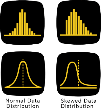
I can show the difference by comparing the histogram of a normal distribution with a non-normal distribution (Figure 1).

Notice that in Figure 1, the histograms on the left column approximate a bell-shaped curve. The top graph depicts data in a sample, where obviously, the number of samples which have the same value or range of values for each sample of the characteristic or variable being investigated, such as age, is plotted.
The graph below it shows the population, where sheer numbers would refine the lines of the curve. Thus, finer lines are obtained.
For example, you may have an age range of 1-5, 5-10, 11-15, 16-20, and so on until the probable age that humans could live. You may arbitrarily place the highest age range which you believe will cover the population you’re interested in.
It would end to something like 96-100 years old. An interval of 5 makes up each bar in the graph.
If you only have, say, a hundred samples, that would show the first graph with rougher edges. While if you sampled a thousand individuals, that would show the refined graph below.
Thus, the graph in Figure 1 at the bottom represents the graph of the population, where more samples were collected. The angled edges of the histogram are no longer visible.
A bell-shaped curved tells us that the researcher must have done the following:
- randomly sampled the population,
- designed the study to consider all members of the population thus be well-represented,
- got a lot of samples, and
- the population or objects of the study comprise a homogeneous group with similar characteristics.
The graphs on the right column skew to the right. These graphs represent a skewed sample and population.
To illustrate further, these graphs would mean that the country where the researcher got the sample has more young generations than the other groups. This population distribution exists in Niger, West Africa, where half of the population is 14 years old or younger.
A non-normal or skewed distribution results when the researcher did the following:
- used purposive sampling in selecting the samples,
- designed the study without due regard to the distribution of the population,
- obtained a few samples, and
- conducted an exploratory survey unsure of the population’s characteristics.
Now, let’s familiarize ourselves with chi square as a statistical test. Who devised this test, what it does, and the requirements to appropriately put the test to use?
Who devised the Chi-Square test?
Karl Pearson, a mathematician, devised the chi-square test. He was the founder of mathematical statistics.
Aside from chi square, Pearson also developed Pearson’s Product-Moment Correlation Coefficient, the popular parametric test to determine the correlation between variables and Principal Component Analysis.
What does the Chi-Square test do?
The chi-square test aims to find out if the frequency distribution of a sample conforms to a theoretical distribution. The theoretical distribution is the expected population distribution of the selected variable under study.
Each interval or span of the histogram, as explained earlier, must be mutually exclusive. Mutually exclusive means that they do not overlap with each other or they could not occur simultaneously.
For example, when a coin is tossed, it would land on either a head or a tail. Not both.
In the example given in the preceding section, that means 1-5 age range is mutually exclusive with the 6-10 age range or 11-15 age range. Or if sex is one of the variables of a study, a male could not be a female. When you ask a person about his or her sex, that person is a male or a female. At least functionally, as there are so-called hermaphrodites.
Thus, the probability of the total events during sampling is 1. If you toss a coin, the probability of a head or a tail when that coin lands on the ground is 50% or 0.50. That’s a simple explanation of probability as a concept of statistics.
If that’s difficult to figure out, view the following video.
Two Types of Chi-Square test comparison
The Chi-Square test assesses two types of comparison namely,
1) tests of goodness of fit that aim to determine if an observed frequency differs from a theoretical distribution, and
2) tests of independence that aim to find out if paired observations are related or unrelated to each other.
Pre-requisites of Chi-Square Test
To avoid faulty or spurious conclusions, you must observe the following rules in using chi square to test for association between the variables of your study:
1. the data should be in the form of frequencies,
2. The data must be independent of each other,
3. there should be over 40 samples in a 2 x 2 (2 rows and 2 columns) contingency table,
4. one or more of the expected frequencies (see formula) is not smaller than 5 in a 2 x 2 table. If the table is larger than 2 x 2, 20% of the cells should have expected frequencies not smaller than 5, and
5. no cell should have an expected frequency lower than 1.
Columns or rows may be merged to get an expected frequency of 1 or higher.
It is assumed that the samples are randomly selected to approximate a normal distribution.
Chi-Square Test Example on Cell Phone Preference
To facilitate the computation of chi square, data must be arranged in rows and columns. I give two examples in the next sections, namely:
- cell phone preference of males and females, and
- soft drink preference of males and females.
Cell phones and soft drinks vary according to the brand while gender will either be male or female. Both are categorical or nominal variables.
Let’s see how data will be arranged for chi square examples 1 and 2.
Frequency Data Table Arrangement
Cell phone preference and gender
Being a member of the product development section of a popular company, you might want to do a marketing research to improve the design of the company’s electronic communication products. Your boss asked you to find out if there is an association between cell phone brands and gender.
The problem question may be phrased this way:
“Is there an association between cell phone preference and gender?”
Given that students are your primary customers, you, as the head of the team, gathered random samples from a large university. Your budget allows the sampling of a thousand students.
To organize the data obtained in the cell phone preference survey, a table may thus see if there is an association between cell phone preference and gender.
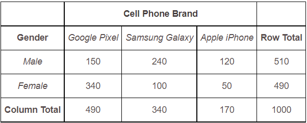
A hypothetical frequency table based on cellphone preference among 1,000 students in a university is given below:
Table 1. Frequency distribution table of cell phone brands and gender.

The values shown in the table show the intersection of the cell phone brand and gender. These values are referred to as the frequency of that intersection. For example, the value of 340 shows females who prefer Google Pixel while 240 shows males who prefer the Samsung Galaxy.
Given the distribution of cellphone preference among students in Table 1, you might be inclined to say that females prefer Google Pixel over the other brands and males prefer Samsung Galaxy. But these results are raw data. It must be analyzed first before making a conclusive statement. Chi square test should be applied first.
The null and alternative hypotheses for this study are as follows:
- Ho: There is no association between cell phone brand and gender
- Ha: There is an association between cell phone brand and gender
As both of the variables are nominal or can be classified into categories, the test to find out if indeed there is an association between gender and cellphone preference is Chi-square.
Chi square formula
The formula for chi square test is written as

where
χ2 – chi square
Oi – observed frequency
∑i – is the expected frequency
However, for our purpose, I simplify the formula into the following descriptive form for clarity on what data goes into those symbols:

where “∑” means you have to sum up or add the difference between the observed value and the expected value, square the difference, then divide by the expected value.
Expected value
The expected value for a cell is computed by multiplying the total frequency of the row with the total value of the column divided by the total number of the samples.
Looking at Table 1, for males who prefer Google Pixel, the expected frequency will be

If we apply the formula for chi square, we can get the following results for all six cells bounded by the rows and columns:

Now, is the computed chi square value significant?
How to determine the significance of the computed chi square value
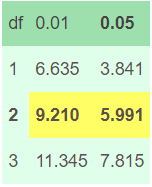
We need to consult a chi-square table and look for the value of chi square at the 1% and 5% level of significance as convention dictates.
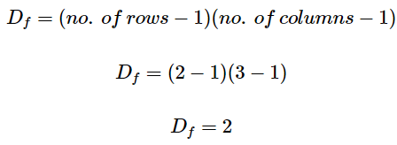
To find the value of chi square using the table, we need to compute for the degree of freedom (Df) for Table 1. Df is computed using the following formula:

Thus, using the chi-square table, we can find the critical chi-square values at the 0.01 and 0.05 levels of significance. These two numbers represent 1% and 5% error that we would allow affirming our hypothesis stated earlier.

I repeat the hypotheses for easy reference:
- Null hypothesis or Ho: There is no association between cell phone brand and gender
- Alternative hypothesis or Ha: There is an association between cell phone brand and gender
The computed chi square value of 159.81 exceeds the tabular value at both the 1% (9.210) and 5% (5.991) level of significance or 159.81 > 9.210 and 159.81 > 5.991, respectively.
Thus, we can have two conclusions for the study using the two levels of significance:
- The data provides sufficient evidence, at the 5% level of significance, that there is a significant association between cell phone brand preference and gender.
- The data provides sufficient evidence, at the 1% level of significance, that there is a highly significant association between cell phone brand preference and gender.
In papers published in scientific journals, values that are significant and highly significant are conventionally applied to an asterisk (*) and a double asterisk (**) after the computed value. Hence, this explains the double asterisk in the computed value of the association between cell phone brand preference and gender.
Practical Uses of the Chi-square test
What are the practical uses of the Chi-square test?
Chi-square test can be used in marketing research. The statistical test can achieve the following research objectives:
- determine if a company’s products sell better in certain locations than others,
- find out if income influences the consumer’s choice of brand,
- discover the relationship between product choice and educational attainment,
- find out if there is an association between day of the week and mall preference, and
- determine if there is an association between race and product brand.
As long as you have two categorical or nominal variables, the best statistical test to apply is the chi-square test.
©2021 November 21 P. A. Regoniel
[cite]
